CustomC estimation engine
The main inbuilt MCMC estimation engine in Stat-JR is known as eSTAT. As explained in Stat-JR’s Advanced Guide it employs an algebra system to construct posterior distributions which can be translated into algorithm steps and from these C++ code is generated to fit the model. This system relies on the ability of the user to specify their model in the form of code that the algebra system can understand. However, since the algebra system has some limitations at present, in the Advanced Guide we describe how, through a preCcode function, we can supplement the output of the algebra system with additional steps. In this current release of Stat-JR we have taken this one step further by introducing a new CustomC estimation engine which circumvents the algebra system completely.
The engine effectively allows the user to work out all the steps for their model algorithm themselves and write these in one Python function that generates C code. Within the ‘Core’ templates we include one such template – 1LevelMVNormalcc. This template fits single level multivariate Normal response models using custom C code and is analogous to the template 1LevelMVNormal. A disadvantage of the 1LevelMVNormal template is the restriction to six responses due to algebra system issues and the use of single site updating steps.
We can set up a model using this template by selecting 1LevelMVNormalcc from the template list and gcsemv1 from the dataset list. Then click on Run and set up the inputs as follows:
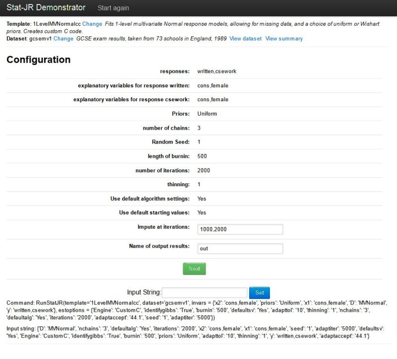
Clicking Next will instantaneously create the C code, as the algebra system isn’t required, and the screen will then look as follows:
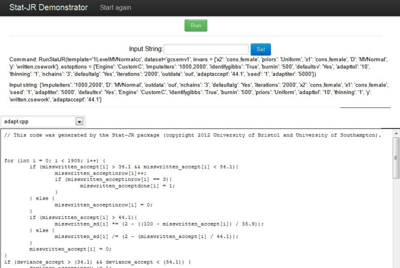
Here you will see that the output pane now fills the bottom of the screen as there are no inputs for this template. Clicking on Run will run this model and give the following if we choose ModelResults from the list:
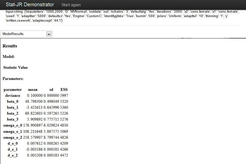
So, from the software user’s perspective, this makes little or no difference to how one interacts with Stat-JR, and so the next section, where we look at the template code, is aimed at template writers who have read the Advanced User guide.
Template Code
As with 1LevelMVNormal, this template has functions invars, preparedata, outlatex and monitorlist, and aside from the removal of one input…
mv = Boolean('Use MVNormal update for beta?: ')
…which is not relevant, here the code in these functions is identical in the two templates.
Near the top of the template code is the engines definition, where we see that the template only works with the CustomC engine:
engines = ['CustomC']
In the packages directory there is a file, CustomC.py, that performs the operations required when the CustomC engine is chosen. This file borrows a lot from eStat.py as, aside from not calling the demo algebra system, the two engines are fairly similar.
The main function in 1LevelMVNormalcc is the function called customccode which contains all the code to fit the model. This function is written in Python but is in effect writing out C code for the update step of the MCMC algorithm: i.e. code to perform 1 iteration of the MCMC algorithm. Steps for adapting (if required) are done automatically by the system and so are not included here. Here we cannot simply write out C code directly as we need to link the code to inputs the user has given. At present this is done throughout the code whereas a C programmer approaching this for the first time might prefer to perform the linking to inputs initially, and then have more generic code; we will investigate this in a later release.
Below we have split the code into chunks in order to comment on each section:
def customccode(self):
        extraccode = '''
        <%!
    def mmult2(names, var, index,count):
        out = ""
        first = True
        for name in names:
            if first == False:
               out += ' + '
            else:
               first = False
            out += 'double(' + name + '[' + index + ']) * ' + var + str(count)
            count += 1
        return out
%>
            {
<% n = len(context['y']) %>\\
Above is the initial chunk which is primarily Python setting up a function that expands out a linear predictor in a model (mmult2) and setting up a Python variable n for the number of responses. We then go on to create code for the first parameter (Omega_e). We start by setting up the two parameters for the update step, sb and vw, with steps that vary depending on the prior.
                // Note currently using a uniform prior for variance matrix
                SymMatrix sb(${n});
                for(int i = 0; i < length(miss${y[0]}); i++) {
<% lenbeta = 0 %>\\
% for i in range(0, n):
                    double e${i} = double(miss${y[i]}[i]) - (${mmult2(context['x' + str(i+1)], 'beta', 'i', lenbeta)});
<% lenbeta += len(context['x' + str(i + 1)]) %>\\
% endfor
% for i in range(0, n):
% for j in range(i, n):
                    sb(${i}, ${j}) += e${i} * e${j};
% endfor
% endfor
                }
% if priors == 'Uniform':
                if (runstate == 0) {
% for i in range(0, n):
                    sb(${i}, ${i}) += 0.0001;
% endfor
                }
% endif
% if priors == 'Wishart':
<%
import numpy
Rmat = numpy.empty([n, n])
count = 0
for i in range(0, n):
    for j in range(0, i + 1):
        Rmat[i, j] = float(R[count])
        Rmat[j, i] = Rmat[i, j]
        count += 1
%>
<% count = 0 %>
% for i in range(0, n):
% for j in range(i, n):
                sb(${i}, ${j}) += ${str(Rmat[i, j] * float(v))};
% endfor
% endfor
% endif
                matrix_sym_invinplace(sb);
% if priors == 'Uniform':
                int vw = length(miss${y[0]}) - ${n + 1};
% endif
% if priors == 'Wishart':
                int vw = length(miss${y[0]}) + ${v};
% endif
                bool fail = false;
                mat_d_e = dwishart(vw, sb, fail);
                mat_omega_e = matrix_sym_inverse(mat_d_e, fail);
Towards the end of the above we see the Wishart call that generates a new value of d_e, the precision matrix, from which a new value of omega_e is generated by inversion. You will see that the if loops for the different priors are in Python and so the C code generated will be specific to the prior chosen. The next code is for the beta parameters:
                // Step for beta
                std::vector betaind(${lenbeta});
<% betacount = 0 %>
% for i in range(0, n):
% for j in range(0, len(context['x' +str(i+1)])):
                betaind[${betacount}] = ${i};
<% betacount += 1 %>
% endfor
% endfor
                std::vector<double*> tmp_x;
% for i in range(0, n):
% for j in range(0, len(context['x' + str(i+1)])):
                tmp_x.push_back((double*)${context['x' + str(i+1)][j]});
% endfor
% endfor
                RectMatrix mat_x(tmp_x, length(${y[0]}));
                std::vector<double*> tmp_ymiss;
% for i in range(0, n):
                tmp_ymiss.push_back(miss${y[i]});
% endfor
                RectMatrix mat_ymiss(tmp_ymiss, length(${y[0]}));
We begin by setting up a few matrices, mat_x and mat_ymiss, that simply place the various predictors and responses into matrix structures for ease of computation. We also construct an indicator variable, betaind, that indicates which response each x variable belongs to.
                SymMatrix db(${lenbeta});
                for (int i = 0; i < length(${y[0]}); i++) {
                    for (int j1 = 0; j1 < ${lenbeta}; j1++) {
                        for (int j2 = 0; j2 < j1+1; j2++) {
                            db(j1, j2) += mat_x(i, j1) * mat_d_e(betaind[j1], betaind[j2]) * mat_x(i, j2);
                        }
                    }
                }
                RectMatrix xtdy(${lenbeta}, 1);
                for (int i = 0; i < length(${y[0]}); i++) {
                    for (int j1 = 0; j1 < ${lenbeta}; j1++) {
                        for (int j2 = 0; j2 < ${n}; j2++) {
                            xtdy(j1, 0) += mat_x(i, j1) * mat_d_e(betaind[j1], j2) * mat_ymiss(i, j2);
                        }
                    }
                }
                fail = false;
                //int err = matrix_sym_invinplace(db);
                //RectMatrix betahat = db * xtdy;
                //mat_beta = dmultnormal(betahat, db, fail);
                RectMatrix betahat = matrix_solve(db, xtdy);
                mat_beta = dmultnormalinv(betahat, db, fail);
The code above then forms the required elements of the posterior distribution and generates new values for beta.
The final section of code, below, performs the update steps for the y variables (if they are missing i.e. if <= -9.999e29). The first section of code creates another indicator vector which maps the starting position of the betas for each response. The y variables that are missing are generated from their univariate normal distributions.
                std::vector betamap(${n});
                int pos = 0;
% for i in range(0, n):
                betamap[${i}] = pos;
                pos += mat_x${i + 1}.cols();
% endfor
% for i in range(0, n):
                for (int j = 0; j < mat_ymiss.rows(); j++) {
                    if (mat_y(j, ${i}) <= -9.999e29) {
                        double tmp = 0.0;
                        for (int k = 0; k < mat_x${i + 1}.cols(); k++) {
                            tmp += mat_beta(betamap[${i}] + k, 0) * mat_x${i + 1}(j, k);
                        }
                        for (int k = 0; k < mat_ymiss.cols(); k++) {
                            if (k != ${i}) {
                                tmp -= mat_d_e(${i}, k) * mat_ymiss(j, k) * (1.0 / mat_d_e(${i}, ${i}));
                            }
                        }
% for m in range(0, n):
% if i != m:
                        for (int k = 0; k < mat_x${m + 1}.cols(); k++) {
                            tmp += mat_d_e(${i}, ${m}) * (1 / mat_d_e(${i}, ${i})) * mat_beta(betamap[${m}] + k, 0) * mat_x${m + 1}(j, k);
                        }
% endif
% endfor
                        mat_ymiss(j, ${i}) = dnorm(tmp, mat_d_e(${i}, ${i}));
                    }
                }
% endfor
            }
         '''
        return extraccode
To see how this code translates into the code generated for the particular inputs in our example we can look at modelcode.cpp in the outputs list; here, ignoring some generic code at the top and bottom, we get:
{
                // Note currently using a uniform prior for variance matrix
                SymMatrix sb(2);
                for(int i = 0; i < 1905; i++) {
                    double e0 = double(misswritten[i]) - (double(cons[i]) * beta0 + double(female[i]) * beta1);
                    double e1 = double(misscsework[i]) - (double(cons[i]) * beta2 + double(female[i]) * beta3);
                    sb(0, 0) += e0 * e0;
                    sb(0, 1) += e0 * e1;
                    sb(1, 1) += e1 * e1;
                }
                if (runstate == 0) {
                    sb(0, 0) += 0.0001;
                    sb(1, 1) += 0.0001;
                }
                matrix_sym_invinplace(sb);
                int vw = 1905 - 3;
                bool fail = false;
                mat_d_e = dwishart(vw, sb, fail);
                mat_omega_e = matrix_sym_inverse(mat_d_e, fail);
                // Step for beta
                std::vector<int> betaind(4);
                betaind[0] = 0;
                betaind[1] = 0;
                betaind[2] = 1;
                betaind[3] = 1;
                std::vector<double*> tmp_x;
                tmp_x.push_back((double*)cons);
                tmp_x.push_back((double*)female);
                tmp_x.push_back((double*)cons);
                tmp_x.push_back((double*)female);
                RectMatrix mat_x(tmp_x, 1905);
                std::vector tmp_ymiss;
                tmp_ymiss.push_back(misswritten);
                tmp_ymiss.push_back(misscsework);
                RectMatrix mat_ymiss(tmp_ymiss, 1905);
                SymMatrix db(4);
                for (int i = 0; i < 1905; i++) {
                    for (int j1 = 0; j1 < 4; j1++) {
                        for (int j2 = 0; j2 < j1+1; j2++) {
                            db(j1, j2) += mat_x(i, j1) * mat_d_e(betaind[j1], betaind[j2]) * mat_x(i, j2);
                        }
                    }
                }
                RectMatrix xtdy(4, 1);
                for (int i = 0; i < 1905; i++) {
                    for (int j1 = 0; j1 < 4; j1++) {
                        for (int j2 = 0; j2 < 2; j2++) {
                            xtdy(j1, 0) += mat_x(i, j1) * mat_d_e(betaind[j1], j2) * mat_ymiss(i, j2);
                        }
                    }
                }
                fail = false;
                //int err = matrix_sym_invinplace(db);
                //RectMatrix betahat = db * xtdy;
                //mat_beta = dmultnormal(betahat, db, fail);
                RectMatrix betahat = matrix_solve(db, xtdy);
                mat_beta = dmultnormalinv(betahat, db, fail);
                std::vector betamap(2);
                int pos = 0;
                betamap[0] = pos;
                pos += mat_x1.cols();
                betamap[1] = pos;
                pos += mat_x2.cols();
                for (int j = 0; j < mat_ymiss.rows(); j++) {
                    if (mat_y(j, 0) <= -9.999e29) {
                        double tmp = 0.0;
                        for (int k = 0; k < mat_x1.cols(); k++) {
                            tmp += mat_beta(betamap[0] + k, 0) * mat_x1(j, k);
                        }
                        for (int k = 0; k < mat_ymiss.cols(); k++) {
                            if (k != 0) {
                                tmp -= mat_d_e(0, k) * mat_ymiss(j, k) * (1.0 / mat_d_e(0, 0));
                            }
                        }
                        for (int k = 0; k < mat_x2.cols(); k++) {
                            tmp += mat_d_e(0, 1) * (1 / mat_d_e(0, 0)) * mat_beta(betamap[1] + k, 0) * mat_x2(j, k);
                        }
                        mat_ymiss(j, 0) = dnorm(tmp, mat_d_e(0, 0));
                    }
                }
                for (int j = 0; j < mat_ymiss.rows(); j++) {
                    if (mat_y(j, 1) <= -9.999e29) {
                        double tmp = 0.0;
                        for (int k = 0; k < mat_x2.cols(); k++) {
                            tmp += mat_beta(betamap[1] + k, 0) * mat_x2(j, k);
                        }
                        for (int k = 0; k < mat_ymiss.cols(); k++) {
                            if (k != 1) {
                                tmp -= mat_d_e(1, k) * mat_ymiss(j, k) * (1.0 / mat_d_e(1, 1));
                            }
                        }
                        for (int k = 0; k < mat_x1.cols(); k++) {
                            tmp += mat_d_e(1, 0) * (1 / mat_d_e(1, 1)) * mat_beta(betamap[0] + k, 0) * mat_x1(j, k);
                        }
                        mat_ymiss(j, 1) = dnorm(tmp, mat_d_e(1, 1));
                    }
                }
            }
For the interested reader you might like to try and match up this code to the Python that generated it. You will see that in various places, in particular in looping, there was the option to perform operations in Python or C. For example you will notice that 2 steps, and hence 2 chunks, of C code are generated for missing values (one for mat_ymiss(j,0) and one for mat_ymiss(j,1)). This is because the for loop was written in Python and so the C code is replicated in slightly modified form rather than having a for loop in C with the modifications in the C code. This makes longer, but probably more readable, C code.
Back to New features.