Individual units may have differential weights attached to them, eg as a result of varying sample selection probabilities from a survey. Thus in a 2 level model we may have differential weights attached to both the level 2 and level 1 units. We first describe the way that weighting was dealt with in MLn.

Weighting in MLn - cautionary note

In MLn a command weight was available. It is also present in MLwiN version 1.0x, but not documented. It applies a simple set of independent weights to each level 1 unit. This gives the same results for the standard regression weighting in single level models but is not really appropriate for multilevel models. In addition there is a bug associated with it which operates in the following way.

In MLn, whenever START or NEXT is typed with batch mode on, then a weight vector(w1) is formed as where w is the column of user supplied weights, typically all less than unity. There is an incorrect line of program code which takes the square root of this newly formed vector. This line of code is executed at every iteration. The repeated taking of the square root moves the weights vector towards the unit vector and the results finally converge at or very close to the unweighted solution.

If batch is turned off and the model is estimated by repeated typing of the NEXT command then at every iteration weights of are used. This is because repeated typing of NEXT resets w1 at each iteration. Thus repeated typing of NEXT with batch off converges to a different solution than running with BATCH ON. By entering the squares of the required weights and using the next command the intended results will be obtained.

MLwiN drives the background MLn server by running an iteration at the time. Hence we will expect different answers with MLwiN run in default mode. The bug does unfortunately mean that MLN weighted analyses in the past were wrong. That is, people would have put in weights found they got very similar or identical answers to unweighted and will have concluded that weights did not make much difference.

A general weighting procedure

The following procedure has been incorporated into release 1.1.

For a description of how to specify a weighted analysis in MLwiN see the weighted model window.

Two cases need to be distinguished. In the first the weights are independent of the random effects at the level. In this case we adopt the following procedure.

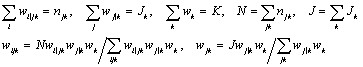
Consider the case of a 2 level model. Denote by the weight attached to the j-th level 2 unit and by the weight attached to the i-th level 1 unit within the j-th level 2 unit such that

      (1)

where J is the total number of level 2 units and the total number of level 1 units. That is, the lower level weights within each immediate higher level unit are scaled to have a mean of unity, and likewise for higher levels. For each level 1 unit we now form the final or composite weight

      (2)

Denote by respectively the sets of explanatory variables defining the level 2 and level 1 random coefficients and form

     (3)

We now carry out a standard estimation but using as the random coefficient explanatory variables.

For a 3 level model, with an obvious extension to notation, we have the following

Denote by the weighting matrix in this analysis. The fixed part coefficient estimates and their covariance matrix are given by

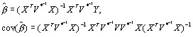      (4)

with an analogous result for the random parameter estimates. MLwiN release 1.1 does not allow the computation of these covariance matrix estimates directly, instead robust or sandwich estimators are used.

The likelihood is evaluated using the weights.

In survey work analysts often have access only to the final level 1 weights . In this case, say for a 2-level model, we can obtain the by computing .

For a 3-level model the procedure is carried out for each level 3 unit and the resulting are transformed analogously.

A number of features are worth noting

First, for a single level model this procedure gives the usual weighted regression estimator.

Secondly, suppose we set a particular level 1 weight to zero.

This is not equivalent to removing that unit from the analysis in a 2 level model since the level 2 (weighted) contribution remains. Nevertheless, this weighting may be appropriate if we wish to remove the effect of the unit only at level 1, say if it were an extreme level 1 outlier. If, however, we set a level 2 weight to zero then this is equivalent to removing the complete level 2 unit. If we wished to obtain estimates equivalent to removing the level 1 unit we would need to set all the level 2 (random coefficient) explanatory variables for that level 1 unit to zero also. This is easily done by defining an indicator variable for the unit (or units) with a zero corresponding to the unit in question and multiplying all the random explanatory variables by it.

In calculating residuals, if you specify weighted residuals then sandwich estimators for standard errors will be used.

This following results (using the notation in Goldstein, 1995) are for weighted residuals for level 2

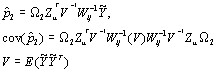     (5)

This provides a consistent estimator of the diagnostic covariance matrix.

The comparative covariance matrix is given by

A similar procedure applies for multilevel generalised linear models. Here the weighted explanatory variables at levels 2 and higher are as above. For the MQL/PQL quasilikelihood estimators at level 1 the vector Zeis that which defines the binomial variation. Thus, for binomial data, at level 1 a method of incorporating the weight vector is to use Z but to work with instead of as the denominator.

The second situation is where the weights are not independent of the random effects at a level. This leads to complications which are discussed by Pfeffermann et al (Pfeffermann, D., Skinner, C. J., Holmes, D., Goldstein, H., et al. (1997). Weighting for unequal selection probabilities in multilevel models. Journal of the Royal Statistical Society, B., 60, 23-40). These authors conclude that, in this situation, the above procedure produces acceptable results in many cases but can give biased results in some circumstances and should be used with caution.

(Back to top)