Residuals
A transcript of Residuals presentation, by Rebecca Pillinger
- To watch the presentation go to Residuals - listen to voice-over with slides and subtitles (If you experience problems accessing any videos, please email info-cmm@bristol.ac.uk)
- See also - Residuals FAQs
Let's begin by revising residuals for a single level model. So in this case, the residual for each observation is just the difference between the value of y predicted by the equation and the actual value of y that we observe. So in other words it's an estimate for the error term e_i.
So, we can write it like this in symbols- y_i hat is the predicted value of y and y_i is the observed value of y
And that means we can calculate the residuals like this, taking the predicted value from the observed value.
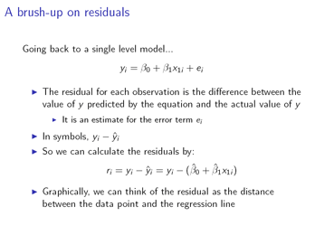
If we want a visual way to think of this, then the residual is simply the distance between the data point and the regression line.
So here we have a graph with lots of data points and a regression line, and if we now add on a couple of residuals, here we have in pinky-purple e_43, that's the residual for observation 43, and you can see that's just the distance between the data point and the regression line, and then over on the left, in green, we have e_20, that's the residual for the 20th observation, and again you can see it's the distance between the data point and the regression line.
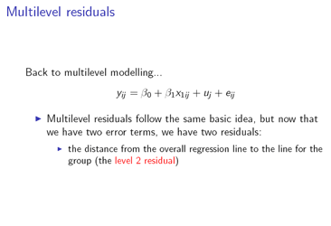
So now, going to the multilevel case, we have the same basic idea, but it's a bit more complicated now, because we have two error terms, so that means we're going to have two residuals: an estimate for u_j and an estimate for e_ij.
So the level 2 residual, the estimate for u_j, is just the distance from the overall regression line to the line for the group.
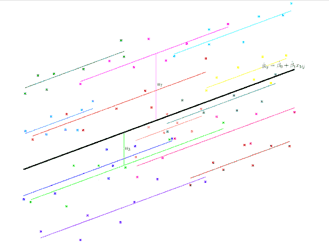
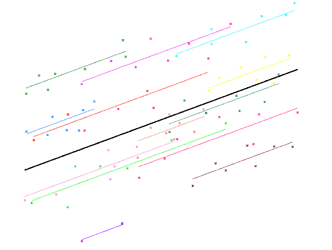
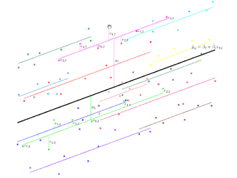
So if we have a look at the graph again, we can imagine that these are exam results, so along the x-axis we have the score at age 11 and on the y-axis we have the score at age 16, and the colours show which school each pupil belongs to, so two points that are the same colour are two pupils from the same school, and we can add in now the lines for each school, and now the level two residuals, so in pinky purple we have u_7, that's the level two residual for school 7, you can see it's the distance between the line for school 7 and the overall regression line, and then in green we have u_3, that's the level two residual for school 3, and again you can see that's the distance between the overall regression line and the line for school 3.

So then the other residual that we have is the estimate for e_ij, the level one residual, and that's the distance from the line for the group to the data point.
So, going back to the graph, we have in pinky purple e_1,7, that's the residual for pupil 1 in school 7, the level one residual, and you can see that's the distance between the data point and the line for school 7, and then in green, we've got e_5,3, that's the level one residual for pupil 5 in school 3, and again you can see that's the distance between the observation for pupil 5 in school 3, and the line for school 3.
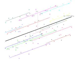
And now if we add in the other residuals for the pupils in those two schools, you can see that in school 7, the pinky-purple school, all of the pupils share the same level two residual, u_7, but they each have their own individual level one residual: e_3,7, e_4,7, e_6,7 and so on. And similarly in the green school, they all share the level two residual, u_3, but they have their own individual level one residuals, e_7,3, e_4,3, e_5,3 and so on. And that's the same for all the other schools.
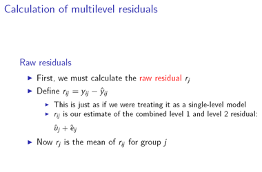
So how do we actually calculate these multilevel residuals? Well, first of all we have to calculate something called the 'raw residual', r_j. And to do that, we define this r_ij- notice that's slightly different, not r_j the raw residual but r_ij, and r_ij is the difference between the observation and the predicted value- it's the distance between the data point and the overall regression line. So that's just the same as for a single level model, just like a single level residual, so far. So r_ij is our estimate of the combined level one and level two residual- it's our estimated u_j plus our estimated e_ij. And r_j, the raw residual, is just the mean of r_ij for group j.
So if we go back to the graph, that's what we've drawn here for this graph: here u_7 is the average distance of the pupils in school 7 from the overall regression line, and u_3 is the average distance of the pupils in school 3 from the overall regression line. And similarly for all the other schools, we've used the average distance to calculate where we should be drawing those school lines.
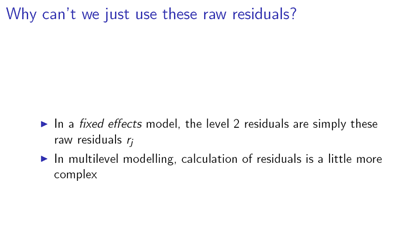
But actually, we don't use these raw residuals as the level two residuals in multilevel modelling. In a fixed effects model, that's exactly what we do: we do take the raw residuals to be our level two residuals. But in multilevel modelling, the calculation of residuals is a bit more complex, and in order to explain why we don't just use the raw residuals, we're going to do a thought experiment.
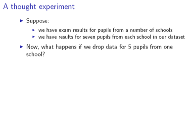
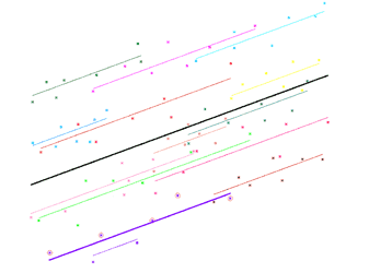
So suppose that we have exam results for pupils from a number of schools, and that we have results for seven pupils from each school in our dataset. So that's just the situation that we've had in the graphs so far.
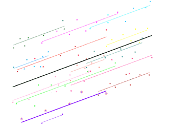
Now suppose that we drop data for 5 pupils from one school, just to see what will happen.
So here we've got a graph showing that; this school down in the bottom now has just two pupils, and we've drawn the fixed effects line using just those two pupils.
But actually, we're much less confident about where we should be drawing that line. We lost a lot of information about the location of the group when we dropped those 5 observations, and it could be that the two pupils that we kept in the dataset are untypical of the school. We're just picking two pupils out of seven, so there's quite a chance that they may be untypical pupils.
So now we're adding back the 5 pupils that we dropped to our graph, so that we can see where they were- we're not adding them back to the model, we're still drawing this fixed effects line using just two pupils that we kept, but we are adding the five pupils back to the graph, so that we can see where they were. And we can see that in fact we did pick two untypical pupils: those two pupils are underneath the other 5 pupils that we dropped.
So now if we put back the fixed effects line using all 7 pupils, we can see that the line using two pupils is actually quite a distance from the line using all 7 pupils, so in a way we can say that the line using two pupils is quite 'wrong'.
So we don't actually have much information about this school, we've only got those two pupils. It turns out that we would therefore do better to combine it with information from the other schools, and it turns out that our best guess is to move the line for this school to lie a bit closer to the overall average for all schools.
So here's the fixed effects line again using just the two pupils, and we actually shrink it in towards the overall average. Here's the fixed effects line, and we shrink it in towards the overall average. And now if we draw those other 5 points again, and the line using all 7 points for that school: here's the fixed effects line using the two pupils, and we shrink it in towards the overall average; here's the fixed effects line and we shrink it in towards the overall average; and you can see that when we do that, it's actually getting closer to the line using all 7 pupils.
Now of course, that needn't necessarily happen. It could be that we had picked two pupils who lay above the 5 that we dropped, or it could be that the 5 we dropped were scattered fairly evenly around the two that we kept. And in those cases, if we shrink the line for the two pupils in towards the overall average, then we'll be moving further away from the line using all 7 pupils, so we'll actually be ending up with a worse guess. But the important point is that the location of the other schools actually tells us something about where those 5 pupils that we dropped are likely to be. The location of the other schools tells us that it's more likely that those 5 points are above the two that we kept, or mostly above the two that we kept, than it is that they're evenly spread around them, or that they're below, or mostly below the two that we kept. So, in other words, it's going to be more likely that, when we move the line for the two pupils towards the overall average, it moves closer to the line for all 7 pupils, than it is that it moves further away when we move it towards the overall average. So, although we might be making a worse guess by moving the line towards the overall average, it's more likely that we're making a better guess by moving it. And that means that the information from the other schools has told us that our best guess for this school is to move the line towards the overall average, to shrink it in.
So that's what our thought experiment has revealed; but actually the same is true for our original dataset. We have only got 7 pupils from each school; there are probably 500 or 1000 really in each school, and so really we don't have very much information about each school. We don't know whether the 7 pupils that we've picked are always typical of their school. So it makes sense in fact to use the same approach: use information from the other groups and shrink the group lines in towards the overall average. And then the level two residuals will be less sensitive to outlying elements of the group.
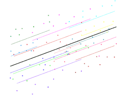
Here are the fixed effects lines and we shrink them in towards the overall average; here are the fixed effects lines and we shrink them in towards the overall average.
Now it's important to say that that's not just because we have only 7 pupils for each school, and that's a very small sample from the 500 or 1000 pupils in the school as a whole: actually with multilevel modelling we will always shrink the group lines in towards the overall average, and that's because we always have a sample, we never have perfect complete information about each group, so we will always do better to use information from the other groups to improve our guess. And of course if we have a lot of pupils from each school - if we have a lot of level one units in each group - then we probably won't shrink the lines by very much, because we do have quite a lot of information already about where the lines should be. So they won't be shrunk very much, but they will still be shrunk a bit.
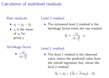
So how do we actually calculate these multilevel residuals? Well, as we said, first of all we need the raw residual, so that's just the mean of r_ij for group j, and the other thing we need is the shrinkage factor, so we calculate that using this formula here: that's the level two variance divided by the level two variance plus the level one variance over the number of elements in the group, n_j. So note that that's going to be not just one constant value for the whole dataset, but a different value for each group, because we have this n_j, the number of elements in each group, changing between groups. So in the example we looked at, with 7 pupils per school, it will actually be the same for each group, because the n_j is the same for each group, it's just 7. But in general, when we can have different numbers of elements in each group, the shrinkage factor will be different for each group, and for example when we dropped 5 pupils and had just 2 pupils in one school, the shrinkage factor for that school would be different to the shrinkage factors for the schools with 7 pupils.
So now we can put those together to get the level two residual, u hat j, by multiplying the raw residual by the shrinkage factor. And you'll be glad to hear that the level one residual is quite simple to calculate once we've done that: it's just the observed value, minus the predicted value from the overall regression line, minus the level two residual.
So if we look at the graph again, here's our observed value; we take away the value predicted from the regression line, and the level two residual, and as expected we end up with this distance as the level one residual.
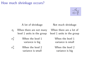
So now let's take a closer look at this shrinkage factor and see how much shrinkage occurs in different situations. So let's think first of all about the number of level one units in the group: is it when we have a lot of units in the group that there is a lot of shrinkage, or when we have not many? Well, in fact it's when there are not many level one units in the group, and that makes sense, because when there are not many level one units in the group, we don't have much information about where that group is located, and so we'll do better to rely more on information from the other groups to tell us where that group is likely to be. But when there are a lot of level one units in the group, then we do have a lot of information about where that group lies, and so we'll do better to rely more on that, and to rely less on information from the other groups.
What about the level one variance now? Is it when that's big that we have a lot of shrinkage, or when it's small? Well, it's when the level one variance is big and again that makes sense, because when the level one variance is big, the individual observations are quite spread out around their group line, and so they're not showing us very precisely where that group line lies, and so we do better to rely more on the information from other groups to tell us where that should be located; but when the level one variance is small, the individual observations are quite tightly clustered around their group lines, and so they show us quite precisely where those group lines are, and so we do better to rely more on those units and less on the information from other groups.
And finally, what about the level two variance? Is it when it's big that we get a lot of shrinkage, or when it's small? Well, it's when the level two variance is small that we get a lot of shrinkage, and again that makes sense, because when the level two variance is small, the group lines are not very spread out around the overall regression line, so that means they're all quite close to each other, and that means that the position of the lines for the other groups tells us quite a lot about where the line for the group we're interested in will be, and so we'll do well to make use of that information quite a lot; but when the level two variance is big, the group lines are quite spread out around the overall regression line, so the position of the other group lines doesn't tell us very much about where the line for the group we're interested in will be, and so we'll do better not to rely on that information so much, but to use the information from the level one units in that group more.
So, just to recap:
We get a lot of shrinkage when there are not many level one units in the group, or when the level one variance is big, or when the level two variance is small; and we get not much shrinkage when there are a lot of level one units in the group, or when the level one variance is small, or when the level two variance is big.