Partitioning variation across levels
- General Normal response models
- Discrete Response models
- Model linearisation (Method A)
- Simulation (Method B)
- A binary linear model (Method C)
- A latent variable approach (Method D)
- Some recommendations
- Variance partitioning in multilevel models for count data
- References
- Sample MLwiN Macros for methods A and B
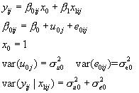
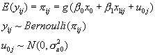
We consider firstly the 2-level variance components model with a single reading test predictor. The model is as follows:
 (1)
(1)
A convenient summary of the 'importance' of schools is the proportion of the total variance accounted for, which we will call the 'variance partition coefficient' (VPC) given by the formula:
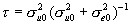
and in the variance components model case this is also a measure of the residual correlation between the responses from two students in the same school, hence the term 'intra-unit correlation' is often found with the use of the symbol  . Researchers involved in multilevel modelling often find it useful to quote an estimate of the VPC and discussions of its usefulness and interpretation often occur on the multilevel email discussion list. This statistic is also known in the sample survey literature as the 'intra class correlation' and is commonly used as a measure of the extent of clustering.
We shall show how this summary statistic can be modified for more complex models when there is no simple decomposition of the overall variance and also in the case where the response variable is discrete.
A more detailed account with examples is given in Goldstein et al.(2002).
General Normal response models
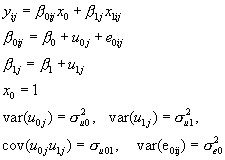
While the VPC is useful for a model such as (1) with a single source of variation at each level, it is less so for a random coefficient model, for example a random-slopes regression model with, say, pupils nested within schools, as follows
 (2)
(2)
Here,

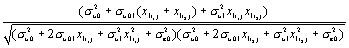
In this case the VPC is not the same as the intra-unit correlation since, for two children with scores  the correlation is given by
Discrete Response models
We shall now consider a multilevel model with a binary response, but our remarks will apply more generally to models for proportions, for different non-identity link functions and also where the response is a count, in fact to any non-linear model. For a (0,1) response, the model that is analogous to (1) is
 (3)
(3)
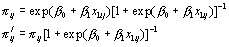
Remembering that the response is just (0, 1), we see that unlike in the Normal case here the level 1 variance depends on the expected value  , as the fixed predictor in the model depends on the reading test score. Therefore as we are considering a function of the predictor variable x1, once again a simple VPC is not available. Furthermore, the level 2 variance,
  , is measured on the logistic scale so is not directly comparable to this level 1 variance.
If we still wish to produce a measure, however, albeit dependent on x1, the following procedures will provide at least approximate estimates.
(Sample macros for implementing these procedures in MLwiN are given at the end)
Model linearisation (Method A)
Using a first order Taylor expansion (see for example Goldstein and Rasbash, 1996) we can write (3) in the form
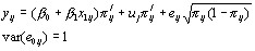
where we evaluate  at the mean of the distribution of the level 2 random effect, that is, for the logistic model
 (4)
(4)
so that, for a given value of x 1we have

and

where sample estimates are substituted.
Simulation (Method B)
This method is general and can be applied to any non-linear model without the need to evaluate an approximating formula. It consists of the following steps:
- From the fitted model (say (3)) simulate a large number m (say 5000) values for the level 2 residual from the distribution
 , using the sample estimate of the variance.
 - For a particular chosen value(s) of x1 compute the m corresponding values of(
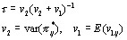
 ) using (4). For each of these values compute the level 1 variance
  .
. - The coefficient is now estimated as
A binary linear model (Method C)
As a very approximate indication for the VPC we can consider treating the (0, 1) response as if it were a Normally distributed variable as in (1) and estimate the VPC as in that case. This will generally be acceptable when the probabilities involved are not extreme, but if any of the underlying probabilities are close to 0 or 1, this model would not be expected to fit well, and may predict probabilities outside the (0, 1) range.
A latent variable approach (Method D)
In some circumstances we may wish to think of an observed (0, 1) as arising from an underlying continuous variable so that a 1 is observed when a certain threshold is exceeded, otherwise a 0 is observed. For the logit model we have the underlying logistic distribution
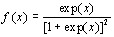 (5)
(5)
with cumulative distribution function
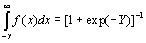 (6)
(6)
The right hand side of equation (6) is simply the logit link function model with Y as the linear component incorporating level 2 variation. The variance for the standard logistic distribution (5) is  so we take this to be the level 1 variance and both the level 1 and level 2 variances are on a continuous scale. We now simply calculate the ratio of the level 2 variance to the sum of the level 1 and level 2 variances to obtain the VPC. A similar device can be used for the probit link function.
This approach may be reasonable where the (0, 1) response is, say, derived from a truncation of an underlying continuum such as a pass/fail response based upon a continuous mark scale, but would seem to have less justification when the response is truly discrete, such as mortality or voting. See also Snijders and Bosker (1999, Chapter 14) for a further discussion.
Some recommendations
In summary, if a VPC is required for non-linear models, it should be computed for a range of values of the predictor variables. Methods A or B are the most appropriate when we wish to measure the variability on the probability scale. Method C becomes unreliable for extreme probabilities. The advantage of method B is that it does not involve any approximation and is simple and fast to compute. We can readily extend the computations for random coefficient models; with method B this simply involves simulating from a multivariate Normal distribution using the estimated level-2 covariance matrix. Method D attempts to measure the variability on an underlying continuous logistic (or Normal) scale and as with continuous response variance component models such as (1) the VPC does not then depend on the values of the linear predictor. If one wishes to make inferences on such an underlying continuous scale then method D is appropriate. The choice of whether to report on the probability scale or an underlying continuous scale will depend on the application; in the example of this paper it seems natural to report directly on the probability scale rather than on an assumed underlying continuous scale of 'propensity' to vote Conservative.
We can obtain an interval estimate for any of our estimates via the bootstrap or using the results from an MCMC estimation run. In the former case we would generate a suitable number (for example 999) bootstrap data sets with associated model fits, and then using one of the above procedures obtain a sample of (999) values from which quantiles can be estimated, as in the first example of the paper. In the MCMC case we would run a chain (of length say 5000) where each MCMC cycle in the chain generates a sample from the posterior distribution of the parameters, and using one of the above procedures this likewise will produce a sample of values from the posterior distribution of the chosen VPC (see Rasbash et al., 2000, Chapter 15).
Variance partitioning in multilevel models for count data
To calculate a VPC for a two-level random-intercept Poisson model see Stryhn et al (2006) and Austin et al (2018)
To calculate the VPC for a Negative Binomial model (that is an over-dispersed Poisson) model see Aly et al (2014) and Leckie et al (2020).
The latter article also considers three-level and random-coefficient extensions to both these models.
References
Bryk, A. S. and Raudenbush, S. W. (1992). Hierarchical Linear Models. Newbury Park, California, Sage: Goldstein, H (1995). Multilevel Statistical Models, Second Edition. London: Edward Arnold.
Goldstein, H., Rasbash, J., Yang, M., Woodhouse, G., Pan, H., Nutall, D., and Thomas, S. (1993). A multilevel analysis of school examination results. Oxford Review of Education, 19, 425-433.
Goldstein, H. and Rasbash, J. (1996). Improved approximations for multilevel models with binary responses. Journal of the Royal Statistical Society, A. 159: 505-13.
Goldstein, H., Browne, W. and Rasbash, J. (2002). Partitioning variation in multilevel models. Understanding Statistics?
Heath, A., Yang, M. and Goldstein, H. (1996) Multilevel analysis of the changing relationship between class and party in Britain 1964-1992. Quality and Quantity 30: 389-404. Rasbash, J., Browne, W. J., Goldstein, H., Yang, M., et al. (2000). A user's guide to MLwiN (Second Edition). London, Institute of Education
Snijders, T. and Bosker, R. (1999). Multilevel Analysis. London, Sage
Aly SS, Zhao J, Li B, Jiang J. (2014) Reliability of environmental sampling culture results using the negative binomial intraclass correlation coefficient. Springerplus [Internet] 3. Available from: http://www.ncbi.nlm.nih.gov/pmc/articles/PMC3916583/
Austin PC, Stryhn H, Leckie G, Merlo J. (2018) Measures of clustering and heterogeneity in multilevel Poisson regression analyses of rates/count data. Stat Med. 20;37(4):572-589. doi: 10.1002/sim.7532
Leckie, G., Browne, W. J., Goldstein, H., Merlo, J., & Austin, P. C. (2020). Partitioning variation in multilevel models for count data. Psychological Methods, 25(6), 787–801. Available from: https://doi.org/10.1037/met0000265 and here.
Stryhn, H., Sanchez, J., Morley, P., Booker, C., & Dohoo, I. R. (2006). Interpretation of variance parameters in multilevel Poisson models. In Proceedings of the 11th Symposium of the International Society for Veterinary Epidemiology an Economics, 702–704. Cairns, Australia. Available at http://www.sciquest.org.nz/node/64294
Sample MLwiN Macros for methods A and B
Methods (C) and (D) are trivial to evaluate. Below are macros for evaluating methods (A) and (B) for any two level binomial model using the MLwiN macro language. The macros require the set of explanatory variable (x) values for which the variance partition coefficient is to be calculated in c151. Column c152 contains the set of x values that have random coefficients in the model. The text for these macros can be executed in an MLwiN macro window. The commands Print b7 or Print b8 display the results from methods A and B in the output window.
Macro for method A
note c151 contains values for set of x variables for which
note: we wish to calculate variance partition coefficient
note c152 contains subset of c151 with random effects at level 2
note calculate (XB) and store in b2 and pi=antilogit(XB) in b3
calc c153=(~c151)*.c1098
pick 1 c153 b2
note calc. Level 2 variance for chosen vals. of expl. Vars: store in b4
calc c153= (~c152) *. omega(2) *. c152
pick 1 c153 b4
note pi^2*Su^2. Su is level 2 variance matrix
calc b3=alog(b2)
calc b5=b3^2*b4
calc b6=b5/(1+expo(b2))^2
calc b7=b6/(b6+b3*(1-b3))
Print b7
Macro for method B
note c151 contains values for set of x variables for which
note: we wish to calculate variance partition coefficient
note c152 contains subset of c151 with random effects at level 2
note calculate (XB) and store in b2
calc c153=(~c151)*.c1098
pick 1 c153 b2
note calc. Level 2 variance for chosen vals. of expl. Vars: store in b4
calc c153= (~c152) *. omega(2) *. c152
pick 1 c153 b4
nran 5000 c154
calc c154=alog(c154*b4^0.5+b2)
aver c154 b1 b3 b2
calc c154=c154*(1-c154)
aver c154 b5 b1
calc b8=b2^2/(b1+b2^2)
Print b8